For measuring the velocity of a projectile, I’m deveveloping a velocity meter. This velocity meter, on which I hope to write some more later on, works by two laser beams that are interrupted sequentially. By measuring the time in between the interruptions, the (average) velocity can be calculated, as the distance between the laser beams is known.
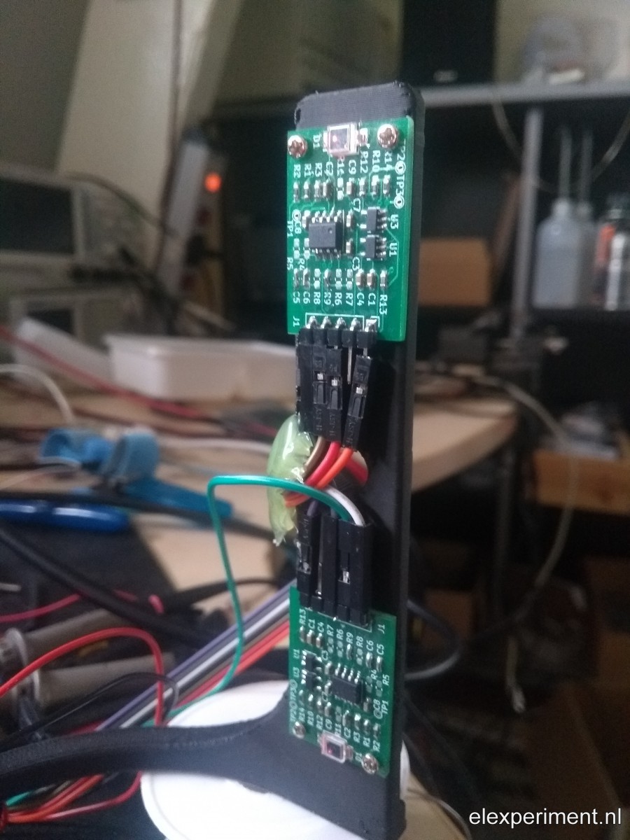
The interruption of a laser beam is measured with a photodiode, with some circuitry behind it, to give it a high optical bandwidth. In the end, a comparator is used, which changes its output if the beam is interrupted. A microcontroller (STM32F103) detects the edges of the comparator outputs, by means of interrupts.
Although the device works, sort of, I want to know whether the device speaks the “truth”. Sure, this can be calibrated by letting an object fall from a given (not too large) height. If the initial height is known, the terminal velocity can be calculated from the relation of potential and kinetic energy. However, what I’m looking for is something different. I’ve noticed, for example, that when firing a projectile, the scope may trigger on spikes in the signal, caused by induced currents. Hence, I want to compare the time domain signals of the comparator outputs (and probably also the analog photodiode outputs), to the output of the velocity meter.
Oscilloscope automation, network setup
The time domain signals of the velocity meter are, of course, measured with the oscilloscope. As I plan to perform many measurements, it’d be nice to automate both signal acquisition and analysis. For this purpose, some Matlab scripts have been developed; of course any other language can be used, as interfacing the scope isn’t too hard.
One warning though: there’s a lot of information, and a lot of methods to be found for communicating with the scope. On the Rigol website, the Ultra Sigma package can be found, containing NI IVI stuff. Another method is to use NI VISA drivers. Both of these options require bulky driver packages; apparently Rigol has been to the school of printer drivers, where they teach to make huge driver packages for a very simple thing.
The simplest solution is to use the SCPI interface, which requires no drivers at all! Just use the LAN connection of the scope, and it works. Many people have already explored this method, see for example: https://hackaday.io/project/5807-driverless-rigol-ds1054z-screen-capture-over-lan
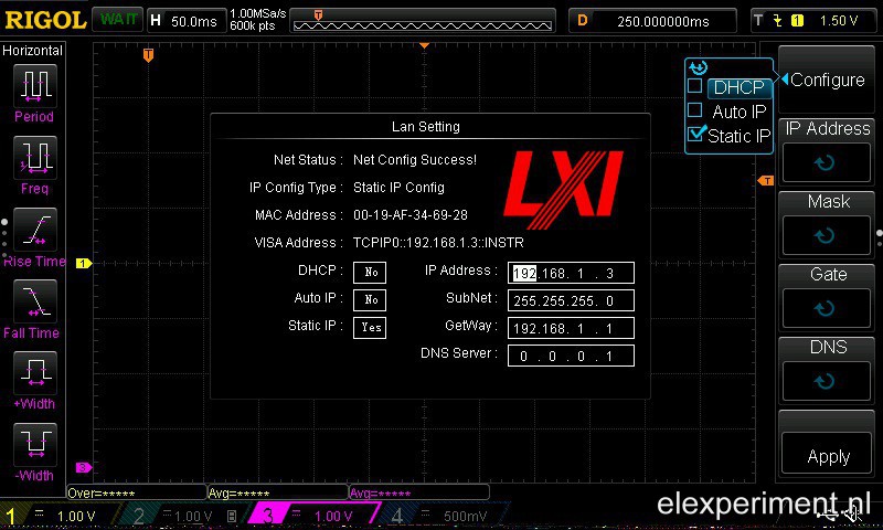
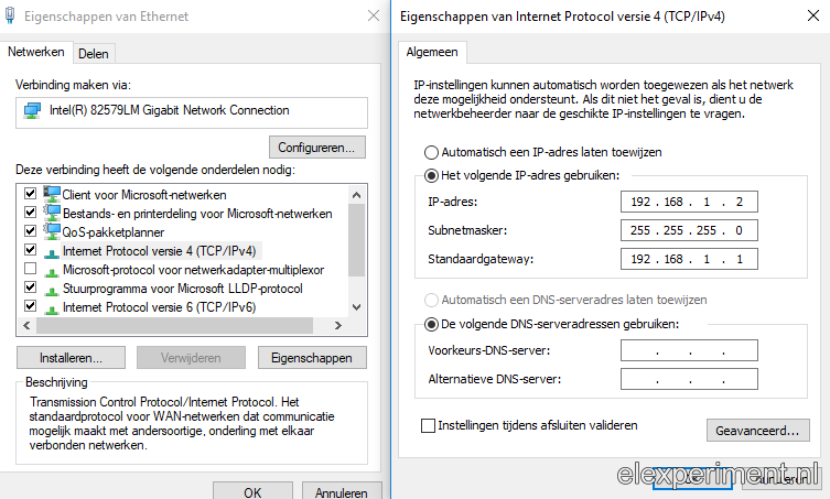
If you connect the scope directly to your router, it will be assigned an IP address via DHCP. You can find the IP assigned IP address using the utility menu on the scope. If you’re for some reason connecting the scope directly to your PC, like I am, you’ll need to configure IP addresses manually. On the PC, see here for an example. For the scope, open the utility menu, choose “IO setting”, “LAN Conf”, to get to the right menu. In there, click “Configure”, and select “Static IP” only. Now, configure the IP address, subnet, and gateway, for example, as follows:
Scope settings
PC settings:
Script time
Now that we have a connection, it’s time to write some scripts! I use Matlab scripts; however, any language can be used, as the only thing that is being done is writing and reading over a TCP/IP interface. I’m using some code from https://github.com/sstobbe/mlab, modified to work with TCP/IP and standard SCPI commands. The link to the adapted code is provided at the end of this post.
An object is simply instantiated with
h = DS1054Z('192.168.1.3');
Then, the approach is as follows: first, the memory depth is set to a relatively small value (300000 points for four channels, twice the value if two channels are enabled). Using the full memory depth would result in very slow data transfers. The correct channel for triggering is automatically set, the edge is set to falling, and the voltage is set to 1.5 V (roughly half of the comparator output, being 3.3 V). The trigger mode is set to single.
h.T_SCALE = 0.05;
h.TRIG_EDGE_CHN = sprintf('CHAN%d', triggerChannelA);
h.TRIG_EDGE_SLOPE = 'NEG';
h.TRIG_SWEEP = 'SING';
h.TRIG_EDGE_LEVEL = 1.5; % Roughly half of 3.3V
The next step is to automatically transfer data, after the velocity has been measured by the DIY meter. The nice part here, is that the velocity meter outputs its measured velocity over the serial port, as well as the measured time between two pulses (for convenience). Matlab listens to the serial port, and as soon as a full line has been received, it will obtain the data from the scope:
</pre>

s = serial(comPort, 'BaudRate', 115200);

h.Single; % Arm scope

fopen(s);

while 1
if s.BytesAvailable>0
l = deblank(fgetl(s));
values = sscanf(l, '%f,%f');
vSer = values(1);
tSer = values(2)/72e6;
break;
end
pause(0.01)
end

fclose(s)
pause(0.5)

% Serial port has given a value, so now scope must contain data
[x,fs,t] = h.WaveAcquire([1 3],0);
And that’s it, that’s how simple it is! Well, after solving the basic bugs, and discovering the bad habits of a Rigol scope, that is.
Time offset
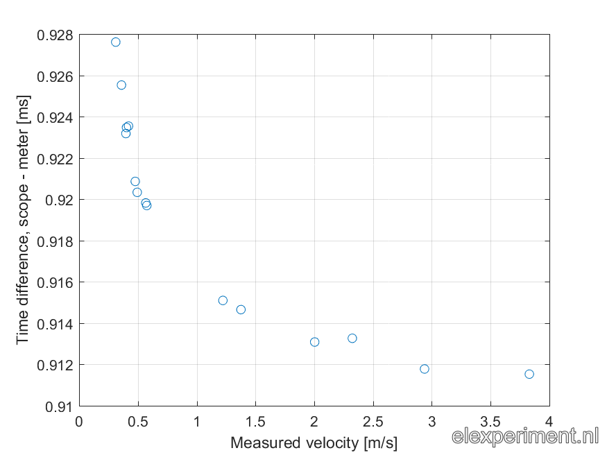
Time for some first measurements! After repeating the above piece of the scripts a number of times, while passing my finger through the meter, and storing the results for each iteration, an array of observations is obtained. Interestingly, the scope and DIY meter give different results, while both simply measure the difference in time between two pulses. Luckily, there’s a pattern: the difference in time between the scope and meter readings is quite constant, as the plot below indicates. Take note: the range of the vertical axis is quite low; the difference in time differences is less than 20 microseconds! So, in short, the DIY meter measures a time that is about 0.9 ms too long. This might not sound like much, but, for the velocities that the meter is intended for, this can produce quite a big error!
When plotting the two time observation sources against each other, a nice plot is obtained:

When performing a linear regression, the dashed line can be plotted. As you can see, the line goes perfectly through all the points, indicating a good linear (or rather, affine) relation between the points. The relation is as follows:

So, both devices return the same time difference very well, up to a constant offset of 910 us. Nice!
Removing the time offset
One way of solving the issue of the 910 us time offset, would be simply to correct for it in software by subtracting a fixed amount of time. That’d be gross however: that’s not a solution, it’s a patch. Let’s look at the code implementation.
void triggerAInt(void) {
  if (timerState==0) {
    timer.resume();
    timerState = 1;
  }
}

void triggerBInt(void) {
  if (timerState==1) {
    timer.pause();

    timeBetweenTrigger = timerCounter*0xFFFF + timer.getCount();

    // Check for too fast reading (caused by EMI spikes)
    if (timeBetweenTrigger<100) {
      timerState = 0;
    } else {
      timerState = 2;
    }
    timer.setCount(0);
    timerCounter = 0;
  }
}

void timerOvfInt(void) {
  timerCounter++;
}
Now, let’s see what we can learn from the offset. The clock rate of the STM32 is 72 MHz. Multiplying 910 us with 72 MHz gives 65520 counts, which is a suspiciously close to 65536. That might look familiar, as it is equal to 2^16. Every time the counter generates an interrupt, 2^16 counts (0xFFFF) have passed. Apparently, after stopping the timer, timerCounter contains a value that is one count above where it should be!
Time to study where this effect originates from. According to the HardwareTimer class documentation, a timer interrupt can be setup as follows:
timer.pause();
timer.setPrescaleFactor(1);
timer.setOverflow(0xFFFF);
timer.setMode(TIMER_CH1, TIMER_OUTPUT_COMPARE);
timer.setCompare(TIMER_CH1, 0x3FFF);
timer.attachInterrupt(TIMER_CH1, timerOvfInt);
timer.refresh();
After diving into the code implementation, this approach gives some problems. The attachInterrupt(timer_channel, interrupt_function_handle) function sets the compare interrupt instead of the overflow interrupt (called update interrupt in STM32 terms). This means an interrupt is generated when the timer counter reaches the value in the compare register for the given channel (1, in this case), set by timer.setCompare. Say, the interrupt is generated when the timer counter reaches 0x3FFF. When the interrupt is generated, the timer counter is not reset to 0, as it is when it reaches its overflow value.
When the timer is stopped, two things can happen: the time can stop before or after the compare interrupt has been generated. If it is stopped before reaching the compare value, both the timer counter and the interrupt counter contain a correct value. However, when the compare interrupt has been triggered, and then the timer stops, the interrupt counter is increased by one, while the timer counter is not reset to zero. Remember: the timer counter starts counting at 0 upon interruption of the first laser beam, and stops counting upon interruption of the second one; it overflows at 0xFFFF every time. So, the “only” thing that goes wrong here, is that the compare interrupt fires at the wrong moment sometimes, leading to a result that is always 0xFFFF counts off from the “true” result, independent of the compare value!
To solve this, we look at the attachInterrupt() function. It appears to directly write the compare channel value (1…4) for enabling a certain compare interrupt to TIM1_DIER register, which looks as follows:
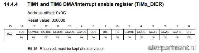
So, the CC1IE (Capture/Compare 1 Interrupt Enable) is set when calling timer.attachIntterupt(TIMER_CH1, timerOvfInt). We want to enable the update interrupt however, located at bit 0. As the attachInterrupt() function doesn’t have any error checking, we simply “hack” it by writing a 0 to it, instead of 1…4. Neat! All this took quite some time to discover; now it works fine though, and I know why!
Now, the measurement of comparing measured time intervals from the DIY meter and scope is repeated. I won’t show the plot again, as it looks virtually the same. The coefficients are now:

That’s a lot of zeroes! The delay is now reduced to 200 ns, which is completely fine with me, as the error it will generate is very small (even at high velocities/short time intervals). The is a difference in “time base” between the scope and DIY meter of roughly 60 ppm, which give a similar error in measured velocity. However, I don’t know which device speaks the truth. Also, I’m quite amazed that the time base of the two devices only differs by such a small amount.
Summary
The purpose of this post was to demonstrate how to easily capture data from a Rigol DS1054Z scope, which is potentially applicable to other scopes as well. Once set up, automated data capture from two measurement methods allows to quickly gather a lot of data. By analysing this data, errors can be quickly discovered. After some debugging, which led a bit to going off topic, the velocity meter now works quite ok.
Resources
The source code can be found in my Git repository: https://gitlab.com/kloppertje/laservelocitymeter
The hardware used in this experiment (photodiodes + high bandwidth amplification) is not yet open sourced, as it is part of another project. In the end, I hope to make this design public as well.